Event-based Method
As stated in previous sections, for the event-based method we will be using spiking jelly to train the raw data, as not only is spiking jelly the only available implementation for non-neuromorphic processors that we have been able to find, but also other implementations of SNN use spiking jelly as a low-level framework.
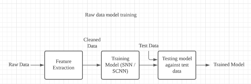
The first step in our implementation is to process the raw data into separate samples shown in our label files. The first step is to create the events_np directory which has a train and test directory within them, both populated by folders for each label, which contain npz files that contain the spike data for each sample. These npz files will be accessed by the model and used to train and evaluate the model. Knowing each raw file at times contains gigabytes worth of spike data, which could lead to multiple tens of millions of lines per raw data file, we need to find a way to load and read the entire file into memory without taking too much time. The default python method of reading these files would have taken a couple of minutes to just load the file into memory, so we chose to use the read_csv method from pandas, which uses NumPy as its low-level framework, which itself uses C to allow fast and efficient array methods. After loading in the CSV file, we save each column as a NumPy array in a dictionary and return that dictionary to be saved.
Once we have gotten a dictionary of the entire raw file, we have to extract each sample and save them to their respective label folder in the train or test set. This is done by finding all events that lie between a range specified by the start_time and end_time columns in our labeling file and saving all the events that lie between that range into a npz file in our events_np folder.
We are able to differentiate between samples that should be in the train set, and samples that should be in the test set by placing the name of the raw file in either trials_to_train.txt or trials_to_test.txt, and these are the files that our preprocessing pipeline uses to process each raw file. After this, we can start to train the model.
We will be training the model for around 100 epochs at most, as each epoch can take up to 10 hours depending on the number of samples you have to train. We will also set the learning rate to 0.001 for our optimizer and encoder. We are using stochastic gradient descent optimization and gaussian tuning encoding.
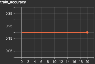
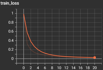
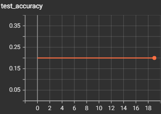
For each epoch, we are first going to train the model, then after training, evaluate the model, so we can see a real-time comparison to see how the model improves at predicting the raw spikes. In each epoch, we loop through each spike in each sample, and send it to the model to train, we increment a counter variable if the spike was predicted correctly, and to see if the PSP calculations threshold was reached, we check if more than 66% of all spikes were predicted correctly, and if they were, then we can say the sample was predicted correctly. We calculate the training loss on how many spikes were predicted incorrectly, and we calculate the training accuracy based on the amount of correctly predicted samples. We repeat the training process for testing but put the model into evaluation mode. After every epoch, we save the model to the directory so we have an updated version after every epoch since each epoch takes a long time to run.


